FGM-3 and FGM-3h magnetometer sensors
General
The Speake & Co Llanfapley FGM-3 and FGM-3h sensors form the basis for the magnetometers used in our observatory. Unfortunately, only basic data is available from the manufacturer on these devices. The basic specifications are given in the table below.
| Parameter | Description |
| Sensitivity | ± 50,000 nT [± 15,000 nT for FGM-3h] at 5 V operating voltage |
| Resolution | Not specified |
| Output waveform | Pulse-width modulated (PWM) |
| Output period | 3 - 25 µs [8 - 16 µs for FGM-3h] |
| Output impedance | Not specified |
| Power | 5 ± 0.5 Vdc, 13 mA: approx. 65 mW |
| Temperature | Not specified |
| Dimensions | 61 mm long (not including pins) x 14.5 mm diameter |
The sensors are 4-terminal devices: Voltage input (5 Vdc), Ground, Signal output, and Feedback as seen in the illustration below
The Feedback pin allows the use of an internal over-wound coil to compensate or null the ambient field. It also could be used to counteract temperature variation effects. It is not used in our applications at this time.
Sensor Output Waveform
The sensor output is a pulse width modulated (PWM) waveform with period proportional to the magnetic induction. The screen shots below show the unloaded output waveform measured with an oscilloscope.
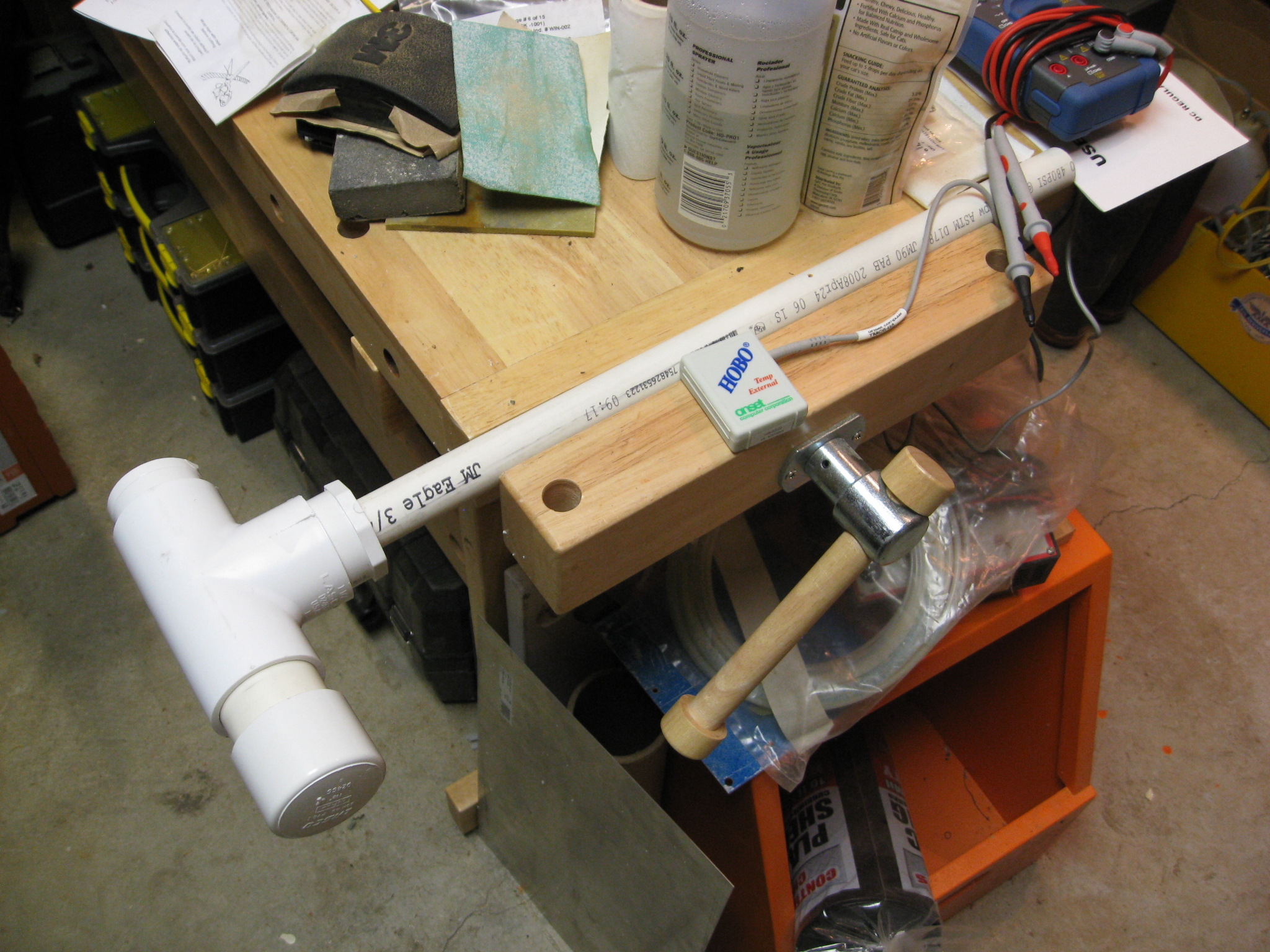
The two charts below show the FGM-3 (upper) and FGM-3h (lower) output waveforms. These measurements were made in the presence of uncontrolled ambient magnetic field and with the sensor fixture vertically oriented on a wood work bench (see accompanying photographs). No effort was made to eliminate or reduce the effects of ferromagnetic objects near the sensor (steel fasteners, tools, power supply, and instrumentation). Both sensors were operating outside of their normal operating range. Since the sensor fixtures each have an on-board voltage regulator, no significant change in the output waveform was detected over a 10.0 to 15.0 V input range.

The photograph below shows two sensor fixtures (middle), one of which is connected to a lab power supply (upper left) and oscilloscope (upper right). The DMM (lower left) measures the input current. Another DMM (not shown) measures the input voltage.

Sensor Output Characteristics
Although these sensors measure magnetic induction, B, in tesla or weber/m2 (1 tesla = 1 weber/m2) the sensitivity curves provided on factory datasheets use magnetic field strength, H, in units of oersted. An alternate unit for magnetic field strength is ampere/meter, where 1 oersted = 103/4π = 79.57747 ampere/meter. For the situation where the sensor is measuring a magnetic field in a vacuum or air, the two quantities are related by B = µ0H, where µ0 is the permeability constant 4π X 10-7 weber/ampere-meter.
The magnetic field strength values on the datasheets can be converted to magnetic induction by multiplying the values in oersteds by [(103/4π) x 4π X 10-7 =] 1 X 10⁻⁴ to obtain values in tesla. For example, the FGM-3 is reasonably linear over a range of approximately -0.7 to +0.7 oersted. Conversion to tesla gives a range of -7 X 10⁻⁵ to +7 X 10⁻⁵ T, or -70 to +70 µT. The FGM-3h is more sensitive than the FGM-3 and is reasonably linear over a range of about -0.15 to +0.15 oersted, or -15 to +15 µT.
For applications where sensor data needs to be scaled by a microcontroller, it is convenient to express the factory data as a simple linear equation even though the input vs output is slightly nonlinear. The two charts below show factory data along with a linear curve-fit and associated equations for the two sensors.
The two charts below show the pulse period output for the FGM-3 (upper) and FGM-3h (lower) as taken from the factory datasheets. Also included is a linear curve fit using the Excel Trendline function. The factory data has not been field verified. The relative sensitivities of the two sensors can be obtained from the slope of the pulse period vs field strength curves. From the factory data, the FGM-3h is about 2.3X more sensitive than the FGM-3 (slope of 0.274 µs/µT and 0.118 µs/µT, respectively).
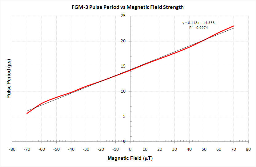
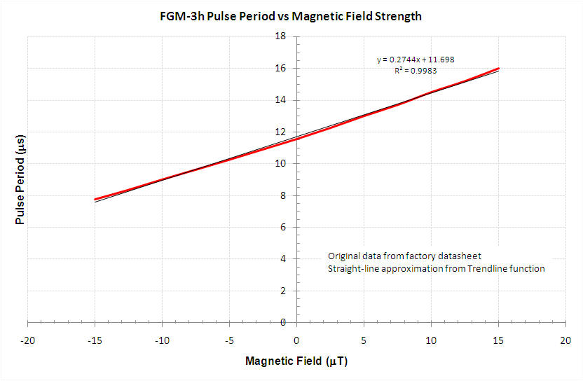
The relative sensitivities of the FGM-3 and FGM-3h can be determined from the slopes of the above Pulse Period graphs. The slope for the FGM-3 is 0.118 µs/µT and for the FGM-3h is about 2.3x as steep at 0.2744 µs/µT. This can be interpreted to mean that for every µT change in field strength, the FGM-3h pulse period changes by 2.3x as much for the FMG-3h.
Sensor Temperature Sensitivity
The FGM-3 sensors are sensitive to temperature changes. We purposely setup a sensor near a baseboard room heater knowing the temperature near it would vary. The temperature varied only fractions of a degree but the sensor output showed visible variations corresponding to the temperature changes. See charts below.
The two charts below show the relative (uncalibrated) output of the FGM-3. The upper chart shows evening data when the temperature is falling and the lower chart shows morning data when the temperature is rising. On the chart for rising temperature, the magnetometer "bottomed out" for its sensitivity setting between approximately 12:45 and 14:45 when the temperature still was falling during the data session. The relevant portions of the chart start around 14:45 when the room temperature started to rise. The temperature data series of both charts reflects the resolution of the temperature sensor, which is a few tenths of a degree. Data were taken at 2 second intervals. Notice that all times are in UTC. Anchorage, AK USA was on Alaska Standard Time (AST), or UTC - 9 hours, when the charts were made (dates shown on horizontal axis).
Sensor Fixtures
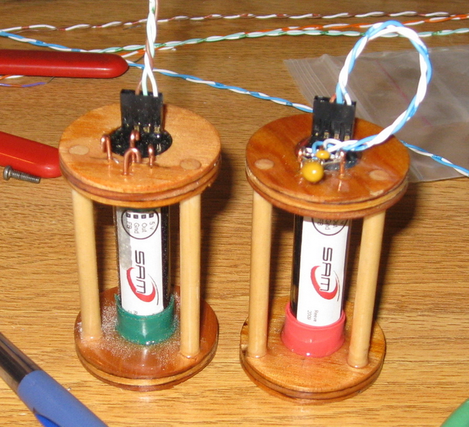
The sensors are mounted in a "monkey cage" (photo below) to provide a rigid mount for the 4-pin SIP connector used to connect the sensor to the sensor cable. Click here for a schematic diagram of the fixture.
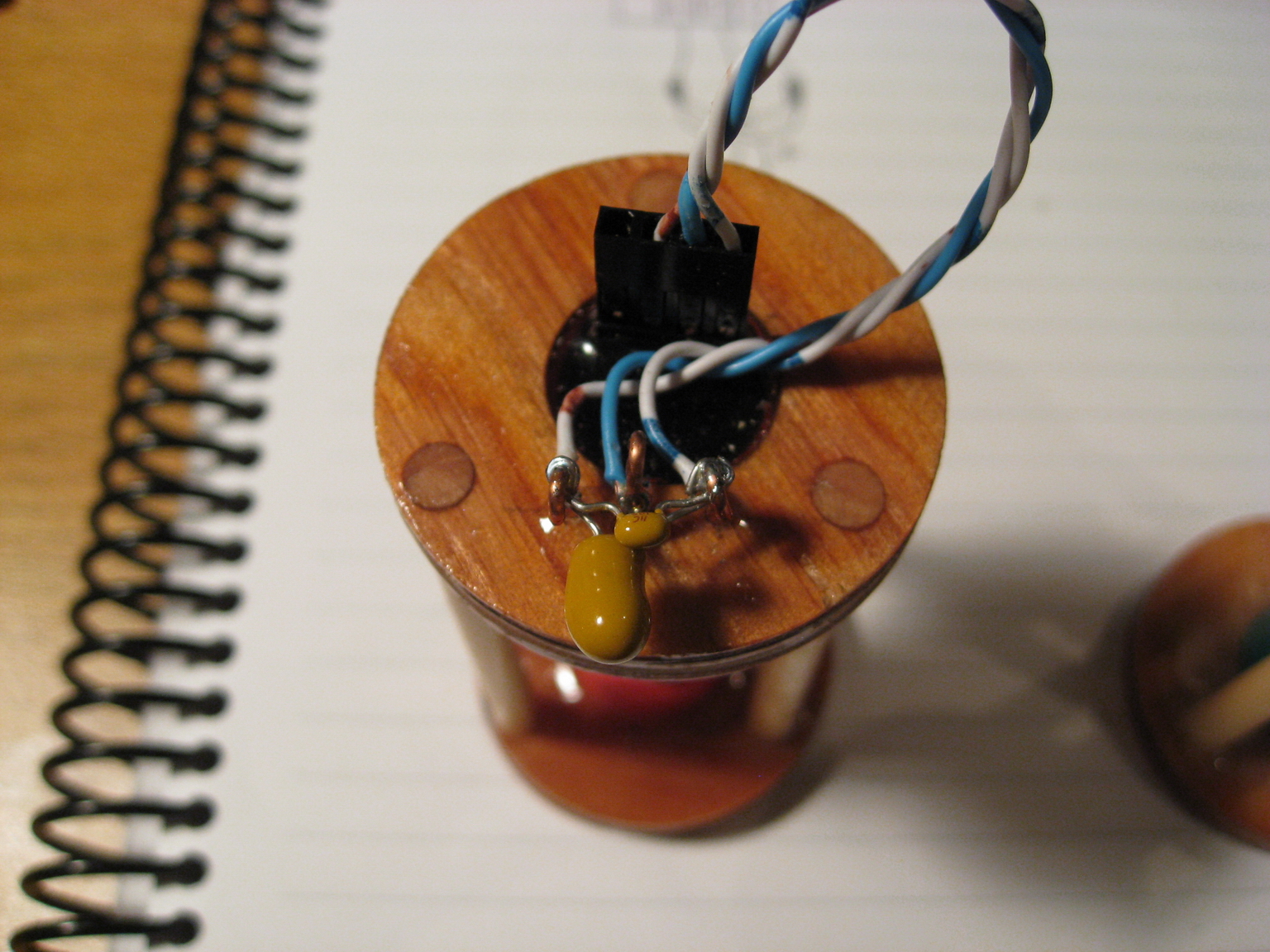
Two types of cages are shown below. One type (left) is all-wood construction and the other is wood and plastic (right). All are glued together with epoxy and wood components finished with a thin epoxy coating. The sensors on the left use solid 18 AWG (1 mm) wire for terminals to hold the voltage regulator and filter capacitors. The wood fixture was drilled and then the wires glued in the holes. Additional wiring details are shown in the before/after images below. The small terminal strips on the sensors shown right are made from phenolic, copper and a small amount of tin and are used on each fixture to rigidly mount and connect the voltage regulator and filter capacitors to the SIP connector.


The monkey cages are designed to slip into a buried fixture made from PVC DWV pipe. Click here for a drawing of the buried fixture. A photograph of the buried fixture is shown below.
The buried fixture assembly is made from common 1-1/2 in. PVC Drain-Waste-Vent (DWV)
pipe (left).
A pipe adapter connects the
1-1/2 in. Tee to 3/4
in. DWV pipe about 50-100 cm long to bring the
power input/signal output cable to a PVC junction box (right) just above the
surface.

Sensor Fixture Input Current
The FGM-3 and FGM-3h sensors are mounted in fixtures. Each fixture includes a linear voltage regulator (LM78L05) and filter capacitors. The local voltage regulator compensates for cable voltage drop in installations where the sensor is some distance from the signal conditioner. The regulator accepts a fairly wide input range and provides a well-regulated output at the sensor utilization voltage (5.0 Vdc). In our application, the system is designed for use with small 12 V valve regulated lead-acid (VRLA) batteries, so the voltage range at the input to the fixture is in the range of 10.0 to 15.0 V. See chart below for input current measurements over this voltage range.
This chart shows the FGM-3h and FGM-3 sensor fixture input currents vs. voltage. It is seen that the FGM-3h, the more sensitive of the two sensor models, has a slightly smaller input current. Both charts include current drawn by the combination of the sensor and the LM78L05 voltage regulator.

The FGM-3 and FGM-3h sensors dissipate about 65 - 70 mW during normal operation, and we are aware of reports that sensor self-heating has caused problems in some installations. Therefore, we tested the buried fixture together with the sensor fixture to measure the temperature rise. The chart below shows the internal and external (ambient) temperatures over a 24 hour period with 14.5 V applied to the sensor fixture.
The sensor temperature rises a couple degrees above ambient and then tracks the ambient temperature throughout the test period (2 days). The ambient temperature shows downward spikes caused by subarctic air entering the shop when the door was opened.

We made temperature measurements with an Onset Computer HOBO model H08-002-02 data logger. The photograph below shows the buried fixture assembly under test in our shop.
The HOBO is visible in the middle of the picture. This data logger has a built-in temperature sensor (channel 1) and provisions for one external temperature sensor (channel 2). We used the Onset model TMC6-HA temperature sensor. It was placed in the buried fixture and lashed with a cable tie to the FGM-3. We used the HOBO's built-in sensor to measure the ambient temperature.
The measurements in the above chart do not truly reflect the thermal performance of the fixture. The measurements were made with the fixture in air and not buried in the earth. In air the heat is carried away from the fixture by convection to the air. In the earth the heat is carried away by conduction to the soil. We expect the heat loss to air to be greater than heat loss to the soil. Even so, based on these measurements, we do not expect problems. The fixture will be buried in the shade and it is unlikely that the soil temperature at depth ever rises above about 15°C.
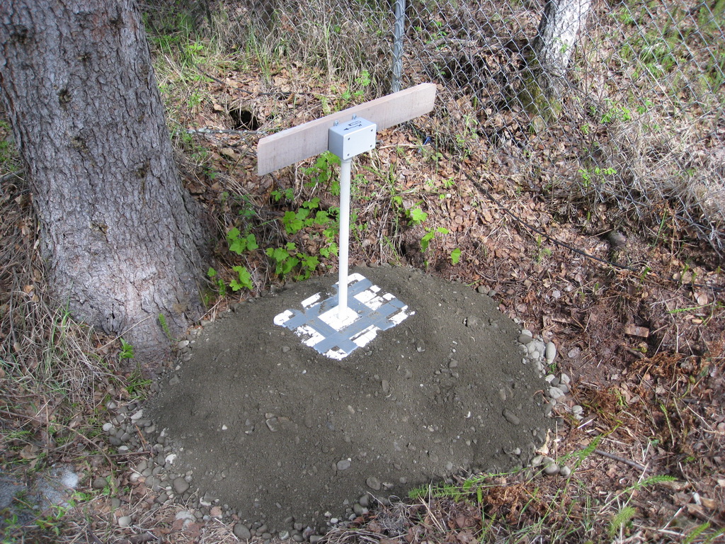
Buried Fixture Installation
To minimize the effects of diurnal temperature variations, we placed the fixture in a Styrofoam picnic cooler, surrounded it with cut-to-fit 50 mm Styrofoam sheets, and then buried the cooler. The following picture sequence shows the installation.
We selected a low shaded area approximately 35 m
north of the shop. After leveling
with rounded rock and sandy soil, we spread about 35 kg of pea-gravel. We
then
placed the cooler, checked its level and orientation (magnetic east) with the
board that was
screwed to the junction box. This fixture uses 100 cm long pipe from the
junction box
to the buried Tee.

We had approximately 0.75 m3 of No. 2
"pit run" sand and gravel delivered nearby.
After removing the larger cobble stones, we slowly buried the cooler by
shuttling the
sand and gravel with a wheel barrow.
After all the sand and gravel was transferred, we
moved the larger rocks
(right side of picture).

We then prepared the cable termination connector.
The cable between the sensor fixture
and the signal processor is 2-pair, 22 AWG shielded twisted pair service cable,
which
we obtained from one of our telecommunications network operator clients. We will
cover
the site with top soil and flowers and build a moose barrier later this summer.

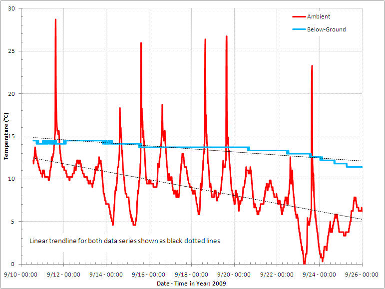
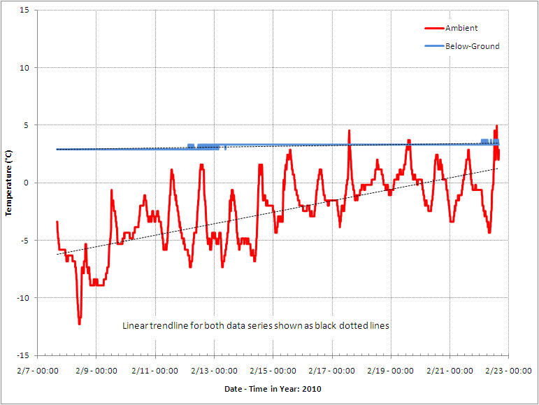
Buried Fixture Temperature Profiles
An Onset Computer TMC6-HA temperature sensor was fed through the above-ground junction box into the conduit and down to the buried fixture. Using the Onset Computer HOBO model H08-002-02 data logger, we measured the ambient (above-ground) and below-ground temperatures in September 2009 and February 2010. The resulting temperature profiles are shown below. In September, the temperature is gradually dropping as shown by the dotted trendline. In February, the temperature is slowly rising as shown by the dotted trendline.
Crosstalk Interference:
When two or three sensors share the same cable back to the SAM-III processor module, there is a good chance of crosstalk interference.
I first noticed this interference in the lab on a cable only 3 m long and found it to be a serious problem in the cable to my buried sensor fixture, which is about 50 m long. John DuBois, a SAM-III user, designed a simple LC low-pass filter that is installed in both our systems and seems to be working well.
Click here for an article that describes the problem and filter and also an alternate fix using separate cables for each sensor.